In a previous Tuesday’s Tip post, we explained what padded zeroes are and how to add them in Excel using apostrophes or by setting the format of the field. Today, we’re sharing an alternative way you can create padded zeros – this time by using a formula. Keep reading to see how you can do this in three easy steps, and (once you’ve got that down pat) how to combine all the steps into one single formula.

Step One

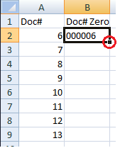
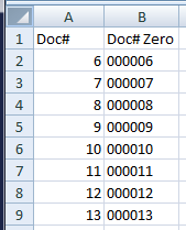
The first step is adding the zeros. To do that, use the “TEXT” function in Excel. In the B2 cell, enter =TEXT(A2,”000000”). This will take the value of the A2 cell and add enough zeros to the front of the number in order to make it six digits:

Step Two

Next, hold and drag the bottom right corner of the C2 cell down the entire column to apply the formula to the rest of the documents. You can also simply double-click on the little square circled above, and it will auto-fill the cells below it.

Step Three

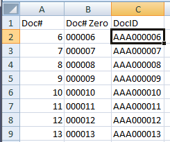
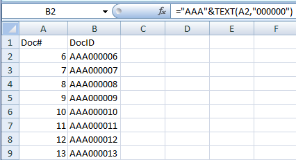
To keep your review organized, you should use a Prefix with each document number. If you skip this step and try to export your DocIDs to Excel, the program will remove all your leading zeros. Your prefix can denote the Custodian of the document, the producing party or even just be a generic prefix such as “AAA” which we’ll use in this example. To add this, use "&" in a formula to combine information from fields and manually entered info. Our DocID field will be in column C and the formula we'll use is ="AAA"&B2”. Again, copy that cell down (as we did in Step 1). You can also enter your prefix in an additional column and use the same "&" function to add two cells together).

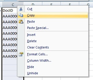
Finally, we want to formulate column C to contain both the prefix and the document numbers together so we’re not left with additional, unnecessary columns. To do this, highlight the entire column (click on the letter C at the top) then right click and select “Copy”:

Leave the column highlighted and right click again. This time select “Paste Values” (the clipboard icon with the numbers 123):

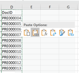
Now you can go ahead and delete your other columns, leaving only the DocID.

Pro Tip

You can do all this in a single step, by combining all the formulas like this ="AAA"&TEXT(A2,"000000"):

The very last step is to save your Excel sheet as a CSV (for Comma Separated Values). Now, you have a load file that will work with most review platforms. Please note, it’s important to be careful if your fields have quotes and/or commas in them, as this can affect how Excel saves out the CSV, and how Review Platforms read the file.

Have any questions? Be sure to let us know in the comment sections below.